Latency Budget Engineering: Where the Milliseconds Actually Go in Live Pipelines

Latency is one of the most visible technical characteristics of modern live media systems. Whether in broadcast production, remote production, live streaming platforms, or interactive media services, latency determines how quickly content moves from capture to audience playback. But in real systems, the harder problem is often not absolute delay alone. It is delay variability: the fact that latency changes from stage to stage, frame to frame, and route to route. That variability is what turns a workable live pipeline into one with AV desync, unstable operator coordination, and timing drift between signals that are supposed to stay aligned.

In many discussions, live latency is treated as one number. In practice, it is the sum of many smaller delays introduced by camera capture, frame processing, encoding, transport, switching, decoding, and playback buffers. Some of those delays are fixed, while others vary depending on codec behavior, jitter, routing, and player buffering. Engineering a live pipeline therefore means more than minimizing delay. It means assigning a budget to each stage and controlling latency variability so the whole chain remains predictable.

Latency budget engineering is the process of analyzing every stage in the chain and assigning timing limits to each one so the overall system meets operational requirements. That approach becomes increasingly important as workflows shift toward IP transport, remote production, and cloud-assisted processing, where extra hops and buffers can easily turn a low-latency design into a fragile one.

The concept of a latency budget

A latency budget defines how much delay is allowed across each stage of the system so the total end-to-end delay stays within target. In a live media workflow, that usually includes capture, production processing, encoding, network transport, switching or orchestration, decoding, and playback buffering.

The key point is that not all stages contribute equally. In professional contribution workflows, capture may cost only a few tens of milliseconds, transport inside a facility may add very little, while encoding, decoding, and packet-jitter handling can add much more. In OTT workflows, playback buffering often dominates the total budget by a wide margin. Regular HLS commonly lands in the 12 to 30 second range, while LL-HLS typically brings end-to-end latency down to about 5 to 10 seconds. Conventional player buffers can also sit around 30 seconds unless deliberately reduced.

Latency budget engineering therefore starts with the operational target. A live sports control room, a REMI workflow, a cloud switching pipeline, and an interactive streaming service all tolerate very different total delays. Once the target is defined, the engineering question becomes where each millisecond is being spent and which parts of that delay are fixed versus variable.

Capture latency in camera systems

The first stage is signal capture, and it already consumes a measurable part of the budget. Camera latency comes from sensor readout, image processing, and internal buffering before the signal appears at the output. Two to three frames of delay inside the camera are common, although high-end systems can do better. In practical terms, that often means tens of milliseconds before the signal even reaches the next stage.

This matters because capture delay is usually a baseline cost, not an exception. Once added, every downstream stage builds on it. And if the video and audio capture paths are not aligned to the same timing reference, even a modest capture offset can become the first step toward visible sync problems later in the chain.

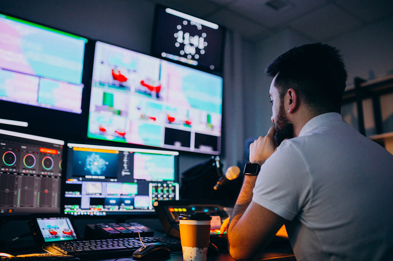
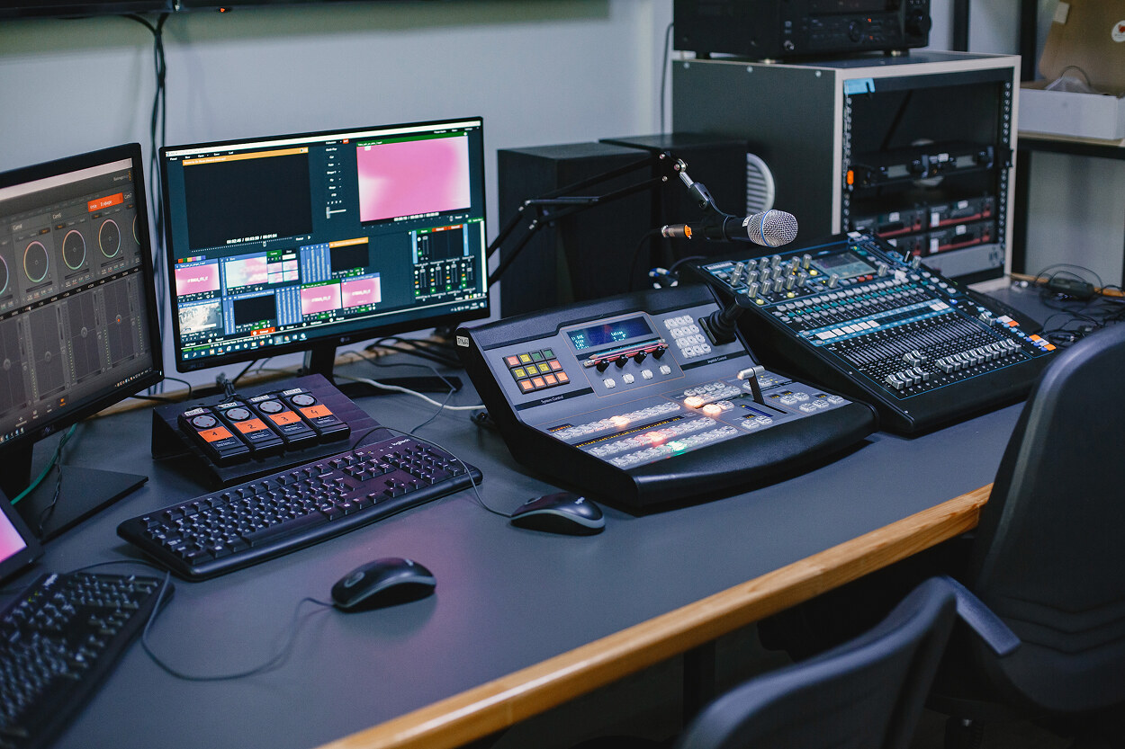
Processing latency in production equipment

After capture, the signal typically passes through production equipment such as switchers, graphics engines, replay systems, multiviewers, processors, and monitoring tools. These stages often look lightweight on diagrams but they frequently add frame-based delay because many video operations are easiest to perform on a full-frame basis.

Video processing in production systems usually incurs one frame of delay or more, and even processes that require only a few lines of latency may still be implemented in frame-based pipelines for efficiency. In a real chain, those single-frame additions accumulate quickly. One frame here and one frame there can become a meaningful part of the total latency budget before encoding or transport even starts.

This is also where latency variability starts to hurt operations. If different signal paths pick up different frame delays, operators are no longer reacting to the same moment in time. That can make switching, replay timing, commentary, and shader response feel unstable even when the total delay is not extreme.

Encoding latency in compressed workflows

Encoding is often one of the largest controllable contributors to latency. Its delay depends heavily on codec choice, GOP structure, lookahead, keyframe interval, and whether the workflow is built for low delay or for efficiency.

At one end of the range, JPEG XS contribution systems are explicitly designed for very low latency, with sub-millisecond codec latency, that is, a fraction of a frame. At the other end, more conventional compressed workflows using AVC or HEVC may add around a frame or more in the encoder alone, and variable encoding complexity can make that delay fluctuate further from frame to frame. The effect gets worse around keyframes and scene changes, where encode time and burst size increase.

Even when the average encoding delay is acceptable, variable encoding latency is dangerous because it feeds jitter into the rest of the chain. A normal P-frame can be ready much sooner than a keyframe, creating a sender-side timing offset before the network has even done anything wrong. That is one reason latency engineering has to track stability, not just averages.

Network transport latency

After encoding, media has to cross a network. In a controlled on-prem environment, transport latency may be relatively small and stable. In distributed live production, remote contribution, or cloud-assisted workflows, it can become both larger and less predictable.

Transport delay includes propagation, switching, routing, queueing, and packet buffering. Inside a facility, the contribution may be only a few milliseconds. Across long-distance REMI or cloud paths, it can easily move into the tens of milliseconds one way, and more importantly, it can vary under load. Fluctuating latency and packet reordering undermine the determinism broadcasters depend on, while larger buffers used to absorb those effects add still more delay.

This is why the problem is often latency variability rather than latency alone. A stable 40 ms transport path is easier to engineer around than a path that swings between 20 ms and 80 ms depending on congestion, switching behavior, or route asymmetry. In timing-sensitive media systems, that variability turns into sync stress downstream.

Switching and orchestration delays

In IP-based production systems, media no longer moves only through fixed physical paths. It passes through switching domains, gateway logic, orchestration layers, and timing-aware control systems. Each of these can add a small amount of delay, and the cumulative effect matters in larger infrastructures.

In ST 2110 systems, the packet path and the timing path both matter. If routing is dynamic, if switches add queueing under load, or if devices operate with different timing assumptions, delay no longer remains purely static. In timing-sensitive IP production environments, asymmetric routing and inconsistent latency can damage synchronization accuracy and lead to jitter, timing drift, or even loss of sync.

These delays are usually smaller than playback buffers or OTT packaging delay, but they are operationally important because they affect determinism. In live production, a few extra milliseconds matter less than whether every related signal experiences the same delay and stays aligned to the same timing model.

Decoding and playback buffering

At the receive side, delay comes from decoding, de-jitter buffering, and playout buffering. In contribution and production workflows, decode plus jitter handling may add from a few milliseconds to a few tens of milliseconds depending on codec, network conditions, and synchronization requirements. In OTT and large-scale streaming, player buffering often dominates the entire latency budget.

Conventional HLS playback can easily run 12 to 30 seconds behind live, while LL-HLS commonly targets 5 to 10 seconds. Low-latency streaming configurations can target under 5 seconds end-to-end, and stream-start latency is directly affected by keyframe interval, with roughly 3 to 4 seconds at 1-second IDR intervals and about 6 to 7 seconds at 2-second intervals.

This stage also exposes the difference between latency and latency variability. Independent audio and video jitter buffers can create playout offsets even if the streams were aligned at the sender. Jitter buffer asymmetry between audio and video is a major cause of sync problems, and drift, encoding asymmetry, and network jitter compound over time.

Latency accumulation across the signal chain

When all stages are combined, total delay becomes the sum of many individually reasonable decisions. A camera that contributes a few frames, a production stage that adds one frame, an encoder tuned for efficiency instead of speed, a WAN path with jitter, and a player buffer sized for resilience can together produce a latency outcome that is far from the original design target.

A useful way to think about this is by range. Capture may consume a few tens of milliseconds. Production processing can add one or more frames per stage. Low-latency contribution encoding and decoding may stay in the low-millisecond to tens-of-milliseconds range, while more conventional compressed or OTT-oriented stages can add far more. Inside a facility the network may be a small part of the budget, but in distributed workflows it can become material. Playback can be modest in contribution monitoring or dominate the budget completely in internet delivery.

That is why latency budget engineering is not just a calculation exercise. It is a bottleneck analysis problem. The job is to identify which stage is consuming too much delay, which stage is adding variability, and which part of the pipeline is making synchronization less stable than the total number alone would suggest.
 

Why deterministic latency matters for live production

In live production, deterministic latency is often more valuable than simply low latency. A system can tolerate delay if that delay is stable and known. It becomes much harder to operate when timing shifts unpredictably between sources, paths, or sites.

The practical consequences are immediate. Variable latency can create AV desync, unstable coordination between director, replay, graphics, and commentary, and timing drift between distributed sources that should remain frame-accurate. Fluctuating delay and loss of symmetry in timing-sensitive networks can lead to significant timing drift, jitter, or even complete loss of sync in ST 2110 environments. Clock drift, encoding asymmetry, and network jitter likewise pull streams apart over time.

For operators, this is not theoretical. When monitors, intercom-linked cues, replay angles, and program outputs do not share a predictable timing model, human coordination gets harder. Even if the audience sees a tolerable total delay, the production team may already be working against an unstable system.

A practical breakdown scenario: remote production / cloud-assisted workflow

A remote production or cloud-assisted workflow makes the latency budget problem easier to see because each stage becomes visible. An illustrative path might look like this: camera capture contributes a few tens of milliseconds, local production processing adds roughly a frame, contribution encoding adds anything from sub-frame JPEG XS latency to tens of milliseconds in more typical compressed contribution, the WAN path adds tens of milliseconds depending on distance and hops, cloud or remote processing adds at least another frame where full-frame operations are used, and decode plus jitter buffering adds another few to several tens of milliseconds before monitoring. If a consumer or OTT player sits at the far end, playback buffering can then overwhelm everything else by adding seconds.

The target for contribution monitoring is obviously much tighter than the target for public OTT delivery. A well-designed remote production deployment can aim for around 250 ms end-to-end including packet-loss recovery buffer, but that only works when each stage is engineered deliberately and variability is tightly controlled.

Where latency engineering connects to Promwad expertise

This is where Promwad’s role should be framed less as general media engineering and more as latency bottleneck analysis and stabilization across real pipelines. In live media systems, the challenge is rarely one isolated delay source. It is the interaction between capture, processing, transport, codec settings, timing design, and playback behavior.

Relevant work here includes latency bottleneck analysis across capture, processing, transport, and playout stages, stabilization of distributed and IP-based media pipelines where variability is causing sync or coordination problems, and system-level integration of video processing, media transport, and playback chains where deterministic behavior matters as much as raw speed. That is particularly relevant in broadcast, Pro AV, remote production, and low-latency streaming systems where small timing errors become visible operational problems.

Why latency budgets are becoming more important in modern media systems

As live media workflows become more distributed, latency budgeting becomes more important and more difficult. Remote production, cloud-assisted switching, packet-based transport, and multi-device playback all add stages where delay can accumulate and where variability can enter.

Without structured latency budgeting, these delays are often discovered only after the system is in operation, when teams start seeing AV desync, inconsistent operator response, unstable timing between sites, or viewers who are much farther behind live than expected. A proper latency budget makes those risks visible earlier by forcing engineers to ask where the delay is, how stable it is, and which stage is responsible for the dominant bottleneck.

That is why modern latency engineering is not just about shaving milliseconds. It is about designing live pipelines that remain predictable, synchronized, and operationally stable as they grow more complex.

AI Overview

Latency budget engineering analyzes where delay is introduced across live media pipelines and how that delay varies from stage to stage. In practice, the engineering challenge is not just lowering total latency, but controlling latency variability so that capture, processing, transport, decoding, and playback remain synchronized and operationally predictable.

Key Applications: live broadcast production, REMI and cloud-assisted workflows, interactive streaming platforms, real-time media transport systems.
Benefits: clearer bottleneck analysis, more predictable timing, better AV synchronization, improved operator coordination, and stronger system stability.
Challenges: balancing compression efficiency against delay, containing playback buffers, managing network jitter, and preventing timing drift across distributed systems.
Outlook: as live media systems become more IP-based, remote, and cloud-assisted, structured latency budgeting will remain essential for keeping complex pipelines synchronized and usable in production.
Related Terms: live streaming latency, broadcast signal chain delay, media pipeline buffering, deterministic media timing, remote production latency, AV synchronization.