


Why Latency Budgets Fail in Industrial Control Systems
Quick Overview
Problem: A latency figure that looks fine on paper — cycle time within spec, network utilisation low, controller “fast enough” — often does not hold once the loop runs under real disturbances, filters and actuator inertia.
Common failure points: Filter phase lag consumed silently in the sensor path, PLC task alignment adding almost a full cycle at worst case, transport modelled as an average, actuator response taken from a datasheet rather than measured under the working envelope.
Where it appears: Multi-axis motion, high-speed packaging and printing, robotics, precision dosing, servo test rigs, and any control loop where a stability margin has to be argued rather than assumed.
Engineering focus: Deriving a worst-case response-time bound from process dynamics, closing the fastest loops locally, using deterministic fieldbus as a bound guarantee rather than a speed figure, and evaluating each stage on the target platform under representative load.
Production Failure Scenario
Wrong Assumption
The assumption that quietly breaks these systems is that a latency budget is a network number. Cycle time, bus load, switch jitter and controller throughput are inputs to the budget — they are not the budget itself. A response-time budget is a bound on the sensor-to-actuator path, derived from what the plant can tolerate. It has to include the stages that rarely appear on a network diagram: filter phase at the loop gain-crossover frequency, sampling alignment inside the controller, and actuator response under load.
Why It Fails
The budget is derived from the wrong end of the loop. Teams start budgeting from the network because it is measurable and familiar. The order should be the opposite: begin at the dominant time constant of the controlled process, choose a stability margin the control law can defend, and allocate the whole response time against that. A high-inertia thermal loop tolerates budgets that would destabilise a servo axis, and the difference is not the fieldbus.
Timing and dynamics are not the same thing. Sampling, transport, scheduling, execution and output staging are additive delays. Filter phase, drive loops and actuator response are dynamic contributions — they shape the loop, not just delay it. Both belong in the response-time story; keeping them on separate lines prevents “we need lower latency” from accidentally meaning “we need less filtering” when the actual constraint is somewhere else. Sensor filtering makes this concrete — every low-pass stage adds phase at the loop gain-crossover frequency, and “add more filtering to reduce noise” is a decision against the stability budget, not against microseconds. This is a signal-chain discipline that belongs to sensor development for industrial environments.
Transport is treated as a mean value. Standard Ethernet with a light load produces usable averages, but without controlled traffic and queues it offers no guaranteed worst-case latency; saturation reveals which one the design assumed. Deterministic fieldbus and industrial Ethernet variants convert transport delay into a bounded service. EtherCAT processes frames on the fly, and the EtherCAT Technology Group cites synchronisation figures at the ≤1 µs level for correctly engineered topologies. PROFINET IRT uses reserved time slots and delivers isochronous behaviour down to sub-millisecond cycles, with the achievable minimum depending on hardware and topology. TSN adds scheduling and shaping primitives that let a shared fabric carry time-sensitive and best-effort traffic together, under a suitable profile such as IEC/IEEE 60802:2026. Whether the transport gives a worst case the loop can hold is a design decision inside industrial network engineering.
Controller scheduling is the term nobody puts on the sheet, and it usually wins. The “PLC scan” mental model — read inputs, execute program, write outputs — hides two effects that dominate in production. The first is sampling alignment: an input arriving just after a task boundary waits nearly a full period before the controller uses it, and that wait is deterministic worst-case, not average. On a 1 ms motion task it can consume close to 1 ms of budget by itself. The second is that execution time is not constant even on a real-time system — cache effects, interrupt service routines and contention with communication stacks add jitter that a mean-based budget systematically underestimates. Engineering this term correctly is the core of custom industrial controller development.
Actuators carry response time that datasheets state generously. Digital outputs and DACs contribute small fixed delays; the actuator itself carries a dynamic response that depends on load, temperature and duty cycle. A servo axis is fast, but its effective bandwidth is set by the current loop and by the mechanical resonance of the load. Pneumatics are slower and pressure-dependent. Hydraulics vary with valve type and oil temperature. If the actuator’s mechanical response is 20 ms, shaving 200 µs off the fieldbus is unlikely to be the dominant improvement — and motor control engineering is where the actuator line stops being an estimate and starts being a measured curve.
Failure Patterns
The following scenarios are representative composites, not individual Promwad case studies.
Scenario 1. A high-speed packaging line runs a 1 ms cyclic control task on a mid-tier PLC. Average cycle time is well inside spec, but a servo axis loses one full period every few hundred cycles: the input mapping runs immediately before the task, and worst-case sampling alignment adds nearly a full period of delay when a disturbance arrives at the wrong moment. The controller is “fast enough”; the loop is not.
Scenario 2. A precision-dosing machine passes commissioning at target throughput. Weeks later, fill accuracy degrades on the third shift and only on the third shift. Instrumenting the response time traces the drift to plant temperature — a proportional valve’s response has moved between cold and warm operation, and the loop was budgeted against the cold number. The fieldbus and the controller are unchanged. The actuator’s bound was never evaluated under the working envelope.
Scenario 3. A multi-axis cell runs its motion on a dedicated EtherCAT segment, with a separate uplink to a shared plant Ethernet for HMI and diagnostics. Motion synchronisation is clean. During a firmware update to a peripheral drive on the plant side, a supervisory session times out intermittently. The motion path is deterministic; the supervisory path shares switch egress on the plant network, and without admission control, shaping or a TSN scheduling policy, the queue behaves as best-effort under bulk load. The application layer runs a retry-then-fail chain that surfaces as a flaky link, and the operator blames the network for a policy gap.
Industrial Control and Real-Time Systems Engineering
Response-time failures in industrial control systems — dropped cycles, phase-margin loss, warm-drift instability, mixed-traffic timeouts — are architecture problems, not networking problems. Closing them takes a bound derived from process dynamics, controller scheduling engineered as a term rather than assumed, and actuator response evaluated under the real operating envelope. Promwad works across industrial controllers, motion firmware, sensor electronics and industrial network integration across EtherCAT, PROFINET, CANopen and TSN, including functional safety software to IEC 61508 where the loop touches a safety case.
Engineering Experience Across Industrial Control and Networking Platforms







Splitting the Loop Across the Platform
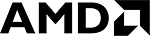
Not every response-time story lives in an incident post-mortem. Some are visible in the architecture of a delivered product. Promwad’s delta robot for high-speed conveyor picking is an example of how the response-time budget can be split across a mixed compute platform.
The delta robot uses an NVIDIA Jetson Orin Nano running Linux + RTOS as the application controller, coordinating three Infineon XMC4800 servo drives over EtherCAT. Motion is layered — position, velocity and current loops sit at their appropriate places in the architecture, with the current loop kept on the drive where it belongs, and higher-level trajectory generation on the application side.
That layering is what a response-time budget usually asks for. The current loop stays close to the motor and the power stage, where its bandwidth is set by electrical parameters rather than by an application scheduler. The velocity and position loops are engineered against the mechanical characteristics of the load. The EtherCAT segment carries the coordination between them as a bounded service. And the application side runs planning, sensing and connectivity without competing for the same time slot as the motion loop.
The takeaway is architectural. When a machine needs a defensible response, the design starts by choosing which loop closes where, and the wire and the scan become terms in that story rather than the story itself.
Solution Approach
Step 1: Anchor the budget in the plant. Take the dominant time constant of the controlled process and the stability margin the control law needs. Fix two numbers: the required update period and the maximum tolerable end-to-end response time. Every other term lives inside those two. A conservative rule of thumb — total response time well under a small fraction of the dominant time constant — is a starting point, not a specification.
Step 2: Separate the timing terms from the dynamics. Budget sampling, transport, scheduling, execution and output staging as additive worst-case delays. Evaluate filter phase, current-loop bandwidth and actuator response as dynamic contributions to the closed-loop response, checked at the loop gain-crossover frequency. Both belong in the story; keep them on separate lines.
Step 3: Treat transport as a bounded service. For deterministic fieldbus and industrial Ethernet — EtherCAT with Distributed Clocks, PROFINET IRT, TSN under a suitable profile such as IEC/IEEE 60802:2026, or CC-Link IE TSN — capture the worst-case cycle for the topology and load the machine will actually run. For any best-effort segment sharing the fabric, isolation needs VLANs and the admission control, shaping or scheduling that make the isolation hold. VLAN tags alone only separate the traffic; they do not schedule it. The choice between EtherCAT, CAN and other field protocols is made against the machine class and the safety story.
Step 4: Build the timing argument for the controller on the target. For hard real-time paths, the argument has to cover WCET, blocking, interference and release jitter across the relevant worst-case conditions. Stress testing on the target under representative load validates that argument, but it does not establish the bound by itself — the bound comes from analysis, and the test confirms it. Priorities, ISR contexts and communication-stack contention have to be considered explicitly, because the numbers move with the SoC, memory subsystem, drivers and kernel configuration. On a Linux-based controller, PREEMPT_RT can reduce scheduling latency substantially, but the achievable bound depends on the platform and workload rather than on a category-level figure — the same discipline applies to any mixed RTOS and Linux industrial architecture.
Step 5: Measure the actuator’s response under the working envelope. Datasheet numbers are best case. Real actuators drift with temperature, load and duty cycle. For servo axes, the current loop is characterised against the electrical parameters of the motor and the power stage, while the velocity and position loops are engineered against a measured mechanical model of the load — not an empty shaft on the bench.
Real Trade-offs
Tightening the control task toward sub-millisecond cycles reduces sampling-alignment delay and improves disturbance rejection, but every reduction squeezes the execution-time margin above it, and can push the compute term into a partitioned architecture where none was needed before. Moving from a 1 ms task to a 500 µs task is a firmware change, not a settings toggle.
Choosing EtherCAT or PROFINET is rarely a raw-timing decision — both deliver bounded cycles for the majority of industrial motion. The trade-off is ecosystem coupling: EtherCAT slots naturally into a machine-builder architecture with Distributed Clocks and CiA 402 drive profiles; PROFINET fits cleanly into a Siemens-centric plant with existing diagnostics and safety patterns; TSN sits where a converged deterministic fabric is being planned across the plant.
Closing the fastest loops locally on distributed drives reduces sensitivity to transport delay and lets the central PLC command setpoints rather than raw control actions. That is cleaner architecture, at the cost of more BOM. Centralising simplifies the controller image, at the cost of a transport bound that has to be tight enough to carry hard control.
Running the hard real-time path on a dedicated core with an RTOS or bare-metal firmware can simplify the timing evidence and interference analysis, but it does not make the design certifiable on its own. It also costs a second compute domain, an IPC layer, and a debug story that crosses two operating systems. On Linux with PREEMPT_RT, the practical worst case depends on the target and configuration — often adequate for industrial products with moderate loops, and always something to be evaluated on the target rather than assumed. The layer is covered in MCU firmware and RTOS engineering.
Typical Response-Time Engineering Tasks

Loop Budget Derivation
Deriving a worst-case response-time bound from process dynamics, allocating it across sensing, transport, compute and actuation, and turning the result into an acceptance criterion.
Motion Control Firmware and Drive Integration
Cyclic control, CiA 402 profiles, distributed-clock synchronisation, and drive integration across current, velocity and position loops.
Real-Time Scheduling on the Target
Task partitioning, RTOS placement, PREEMPT_RT configuration on Linux industrial controllers, and evaluating execution-time bounds against real workloads on the target.
Sensor Path and Filter Engineering
Analogue front-end design, ADC selection and sampling architecture, and keeping filter phase contribution explicit at the loop gain-crossover frequency.
Deterministic Fieldbus and Industrial Network Integration
EtherCAT, PROFINET IRT, TSN and CC-Link IE TSN engineering, cycle-time and topology design, and traffic isolation for mixed motion, diagnostic and update fabrics.
Qualifying Symptoms
- Motion axes miss occasional cycles or overshoot on outliers while average cycle time reports inside spec.
- Servo behaviour that held on the bench degrades on the machine, correlated with sensor filtering changes or shared communication load.
- Diagnostic or supervisory sessions time out intermittently under normal operating traffic on a nominally deterministic fabric.
- Actuator response drifts with temperature or duty cycle, and the loop was budgeted against a datasheet value rather than a measured one.
- The controller’s timing argument has never been built for the target under ISR and communication-stack contention.
- Software filtering was added to a noisy sensor path and quietly cost stability margin at the loop crossover.
- The response-time budget is reported as a single average — no upper bound, no jitter reserve.
Solution Context Link
At this point the work is closed-loop architecture, not another network upgrade. In practice: a budget anchored in process dynamics, transport modelled as a bounded service, a timing argument for the controller built on the target, and actuator response measured under the working envelope.
For machines whose loops cross into a safety case, the same discipline feeds directly into IEC 61508 functional safety software — a bound argued for the target platform is a prerequisite for a safety case, not an optimisation on top of it. Where the fabric is shared with slower plant-network traffic, the industrial network engineering layer is where isolation and traffic-class boundaries are engineered rather than assumed.
FAQ
How do you build a response-time budget for an industrial control loop?
Why is PLC scan time often the dominant term?
Is p99 the right metric for a hard real-time control loop?
When does faster networking not help?
Which industrial networks fit hard real-time motion?
Does the choice of RTOS or Linux configuration matter?
Related Engineering Cases
- Reusable Robotics Software Platform (EtherCAT + ROS 2 + 5G on Qualcomm RB3 + Hilscher netX 90): Reusable embedded robotics stack combining EtherCAT motion control on Hilscher netX 90 with FOC and CiA 402 profiles, multi-axis BLDC control, ROS 2 integration via ros2_control, and 5G remote operation, packaged as a Yocto image. Relevant to fast/slow-loop partitioning and to keeping motion inside its own timing domain.
- Delta Robot Design for Conveyors (NVIDIA Jetson Orin Nano + Infineon XMC4800 + EtherCAT): Custom delta robot with Linux + RTOS on Jetson Orin Nano and XMC4800-based servo drives over EtherCAT, with position, velocity and current loops layered across the platform. An example of splitting the response-time budget across an application controller and dedicated drives.
- AC/DC Servo Drive Development: Hardware, software and enclosure for a production-oriented AC/DC servo drive supporting position, torque, velocity and full-closed control, with EtherCAT and CANopen and incremental or absolute encoder feedback — the drive-level layer where actuator response is engineered.
Find the Bottleneck in Your Control Loop